| Laplace Transforms of Functions |
The Laplace transform converts a function of a real variable, which is usually time t, into a function of a complex variable that is denoted by s. The transform of f (t) is represented symbolically by either ℒ[ f (t)] or F(s). One can think of the Laplace transform as providing a means of transforming a given problem from the time domain, where all variables are functions of t, to the complex-frequency domain, where all variables are functions of s.
The defining equation for the Laplace transform is:
Eq1 defines the one-sided Laplace transform. There is a more general, two-sided Laplace transform which is useful for theoretical work but is seldom used for solving for system responses. Sometimes the lower limit of integration is made at t = 0− rather than at t = 0. Either convention is acceptable provided that the transform properties are developed in a manner consistent with the defining integral.
The integration in Eq1 with respect to t is carried out between the limits of zero and infinity, so the resulting transform is not a function of t. In the factor ε−st appearing in the integrand, s is treated as a constant in carrying out the integration.
The variable s is a complex quantity and follows the form of Eq2 from the lesson Complex Numbers, Real and Imaginary:
s = σ + jω
where σ and ω are the real and imaginary parts of s, respectively. The factor ε−st in Eq1 can be written as:
ε−st = ε−σ t ε−jωt
Because the magnitude of ε−jωt is always unity, |ε−st| = ε−σ t. By placing appropriate restrictions on σ, it can be ensured that the integral converges in most cases of practical interest, even if the function f (t) becomes infinite as t approaches infinity. For most time functions considered, convergence of the transform integral can be achieved.
The Laplace transforms of some common functions will now be derived. The following results, along with others, are located in the reference Laplace Transforms of Functions.
Step Function
Suppose f (t) has a constant value A for all t > 0. Because the range of integration in Eq1 is over only positive values of t, the transform of f (t) is not affected by its values before t = 0. Then it follows from Eq1 that:
In order for the integral to converge, |ε−st| must approach zero as t approaches infinity. Because |ε−st| = ε−σt, the integral will converge, provided that σ > 0. Hence the expression for the transform of this function converges for all values of s in the right half of the complex plane, and Eq2 becomes:
Note that the variable t has disappeared in the integration process and that the result is strictly a function of s.
For all functions of time which will be of concern, the transform definition will converge for all values of s to the right of some vertical line in the complex s-plane. The region of convergence may be required in some advanced applications, but will not be covered here. When evaluating Laplace transforms, it shall be assumed that σ, the real part of s, is sufficiently large to ensure convergence.
The unit step, denoted by U(t), is an important function. Note that a capital letter U is used, in contrast to the lowercase letter in the symbol u(t) for a general input. The unit step function is defined to be zero for t < 0 and unity for t > 0. Its Laplace transform is given by Eq3 with A replaced by 1. Thus,
Exponential Function
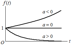
Depending on the value of the parameter a, the function f (t) = ε−at represents an exponentially decaying function, a constant, or an exponentially growing function for t > 0, as shown:
In any case, the Laplace transform of the exponential function is:
| ℒ | [ε−at] = | ∫ | | ε−atε−stdt = | ∫ | | ε−(s + a)tdt = | | | |
The upper limit vanishes when σ, the real part of s, is greater than −a, so:
Note that if a = 0, the exponential function ε−at reduces to the constant value of 1. Likewise, Eq5 reduces to Eq4, as it must for this value of a.
Ramp Function
The unit ramp function is defined to be f (t) = t for t > 0. Substituting for f (t) in Eq1:
To evaluate the integral in Eq6, the formula for integration by parts is used:
where the limits a and b apply to the variable t. Making the identifications u = t and v = ε−st/−s, a = 0, and b → ∞, Eq6 can be rewritten as:
It can be shown that:
provided that σ, the real part of s, is positive. Thus:
Because the integral in Eq7 is ℒ[U(t)], which from Eq4 has the value 1/s, Eq7 simplifies to:
Trigonometric Functions
When f(t) is replaced by sin ωt or cos ωt in the definition of the Laplace transform, the resulting integral can be evaluated by using the identities in the Trigonometric Identities reference, by performing integration by parts, or by consulting a table of integrals. Using an integral table, it is found that:
| ℒ | [sin ωt] = | ∫ | | sin (ωt) ε−st dt = | | (−s sin ωt − ω cos ωt) | | | = | |
By a similar procedure, it can be shown that:
Rectangular Pulse
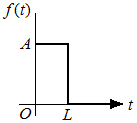
The rectangular pulse shown in the following figure has a height of A and a duration of L.
Its Laplace transform is:
| (Eq8) | | F(s) = | ∫ | | Aε−st dt + | ∫ | | 0ε−st dt = | | ε−st | | | + 0 = | | (1 − ε−sL) |
|
When A = 1 and when the pulse duration L becomes infinite, the pulse approaches the unit step function U(t). Also, the term ε−sL in Eq8 approaches zero for all values of s having a positive real part. Under these conditions, F(s) given by Eq8 approaches 1/s, which is ℒ[U(t)] as expected.